ChatGPT, which came out at the end of 2022, shocked the Internet. It can’t help but remind people of AlphaGo in early 2016, challenging the story of Li Shishi, the top human Go master. In a popular science book on probability published in 2017 [1] , I gave a brief description of the state of artificial intelligence at that time. It was the second revolution of AI, and deep machine learning and natural language processing (NLP) had just started. Unexpectedly, just a few years later, the third wave of AI came rolling in, which basically solved the problems of understanding and generating natural language. With the release of ChatGPT as a milestone, it opened up a new era of natural human-computer communication.
The idea of artificial intelligence (AI) has been around for a long time. British mathematician Alan Turing, not only the father of computers, also designed the famous Turing test, which opened the door to artificial intelligence. Today, the application of artificial intelligence has penetrated into our daily life. Its successful rise stems from the rapid development of computers, the rise of cloud computing, the advent of the era of big data, and so on. Among them, the mathematical basis related to big data is mainly probability theory. Therefore, this article will talk about an aspect of ChatGPT related to probability, and more specifically, it is related to a name hundreds of years ago: Bayesian.
Probability Theory and Bayesian
Regarding probability theory, Laplace (1749-1827), known as the French Newton, once said:
“This science derived from the gambling machine will surely become the most important part of human knowledge. Most of the problems in life will be just a matter of probability.”
Today’s civilized society more than two hundred years later has confirmed Laplace’s prophecy. This world is full of uncertainties, probabilities everywhere, and everything is random. There is no need for an abstract definition. The basic intuitive concepts of probability theory have already penetrated into people’s work and life. From the small lottery tickets that everyone can buy, to the stars and the universe, to the complexity of computers and artificial intelligence, they are all closely related to probability.
So, who is Bayesian?
Thomas Bayes (Thomas Bayes, 1701-1761) was an English mathematician and statistician in the 18th century. He used to be a priest. However, he was “unknown during his lifetime, but worshiped by everyone after his death”, and he became “popular” in the contemporary science and technology circle. The reason is attributed to the famous Bayes theorem named after him. This theorem has not only contributed to the development of the Bayesian school in history, but is now widely used in machine learning, which is closely related to artificial intelligence [2] .
What did Bayes do? Back then, he studied the probability problem of a “white ball and black ball”. Probability problems can be calculated forward and backward. For example, there are 10 balls in a box, black and white. If we know that out of 10 balls, 5 are white and 5 are black, then, if I ask you, what is the probability that a ball is randomly drawn from among them to be black? The question is not difficult to answer, of course it is 50%! What if 10 balls are 6 white and 4 black? The probability of drawing a ball to be black should be 40%. Consider a more complicated situation: If 2 white and 8 black out of 10 balls, now randomly pick 2 balls, what is the probability of getting 1 black and 1 white? There are 10*9=90 possibilities to get 2 out of 10 balls. There are 16 cases of 1 black and 1 white. The probability is 16/90, which is about 17.5%. Therefore, we only need to perform some simple permutation and combination operations, and we can calculate the probability of taking n balls out of which m are black balls under various distribution situations of 10 balls. These are examples of counting probabilities forward.
However, Bayesian was more interested in the reverse “inverse probability problem”: Suppose we don’t know the ratio of the number of black balls and white balls in the box in advance, but only know that there are 10 balls in total, then, for example, I Take out 3 balls at random and find that they are 2 black and 1 white. The inverse probability problem is to guess the proportion of white balls and black balls in the box from this test sample (2 black and 1 white).
The “inverse probability” problem can also be illustrated from the simplest coin toss experiment. Suppose we don’t know whether the coin is fair on both sides, that is, we don’t know the physical bias of the coin. At this time, the probability p of getting heads is not necessarily equal to 50%. Then, the inverse probability problem is an attempt to guess the value of p from a certain (or several) experimental samples.
To solve the inverse probability problem, Bayes provides a method in his paper, Bayes’ theorem:
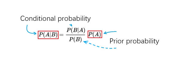
P(A|B) = (P(B|A) * P(A))/ P(B) (1)
Here, A and B are two random events, P(A) is the probability of A happening; P(B) is the probability of B happening. P(A|B) and P(B|A) are called conditional probabilities: P(A|B) is the probability that A occurs when B occurs (condition); P(B|A) is the probability that A occurs The probability of occurrence of B in the case of .
Examples of applying Bayes’ theorem
Bayes’ theorem can be interpreted from two perspectives: one is “expressing the mutual influence of two random variables A and B”; the other is “how to correct the prior probability to obtain the posterior probability”, which are illustrated with examples below.
First, roughly speaking, Bayes’ theorem (1) involves two random variables A and B, representing the relationship between two conditional probabilities P(A|B) and P(B|A).
Example 1: The law and order in a small town was not very good in January, and there were 6 robberies within 30 days. The police station has a siren that goes off when something happens, including natural disasters such as fires and storms, and man-made disasters such as theft and rape. In January, the siren went off every day. And, from past experience, if a resident is robbed, the probability of the siren going off is 0.85. Now that the siren is heard again, what is the probability that the sound represents a burglary?
Analyze this question. A: burglary; B: pull the alarm. Then, we know (January):
Probability of burglary P(A) = 6/30 = 0.2; probability of raising the alarm P(B) = 30/30 = 1; P(B|A) = probability of raising the alarm during burglary = 0.85.
Therefore, according to the formula (1), substituting the known 3 probabilities, the calculation results in P(A|B) = (0.85*0.2/1) = 0.17.
That is to say, the probability that “the alarm sounded because someone broke into the house” this time is 17%.
The following example illustrates how to use Bayes’ theorem to calculate “posterior probability” from “prior probability”. First rewrite (1) as follows:
To summarize (2) in one sentence, it says: Using the new information brought by the occurrence of B, the “prior probability” P(A) of A can be modified when B does not occur, so as to obtain the occurrence (or existence) of B , the “posterior probability” of A, that is, P(A|B).
First, let’s briefly illustrate with an example given by Daniel Kahneman, an American psychologist and winner of the 2002 Nobel Prize in Economics.
Example 2: There are two colors (blue and green) of taxis in a city: the ratio of blue cars to green cars is 15:85. One day, a certain taxi hit and ran away at night, but there happened to be an eyewitness at the time, who believed that the taxi that caused the accident was blue. But what about his “credibility of witnessing”? The public security personnel conducted a “blue-green” test on the witness in the same environment and obtained: 80% of the cases were correctly identified, and 20% of the cases were incorrect. The problem is to calculate the probability of the car that caused the accident being blue.
Assume that A=the car is blue, and B=witnessed blue. First we consider the base ratio (15:85) of the blue-green taxi. That is to say, in the absence of witnesses, the probability of the car causing the accident being blue is 15%, which is the prior probability P(A)=15% of “A=blue car causing the accident”.
Now, having a witness changes the probability of event A occurring. Witnesses saw the car as “blue”. However, his witnessing ability is also compromised, with only an 80% accuracy rate, which is also a random event (denoted as B). Our problem is to ask for the probability that the car involved in the accident is “really blue” under the condition that the witness “sees the blue car”, that is, the conditional probability P(A|B). The latter should be greater than the prior probability of 15%, because the witness saw the “blue car”. How to fix the prior probability? P(B|A) and P(B) need to be calculated.
Because P(B|A) is the probability of “sighting blue” under the condition of “the car is blue”, that is, P(B|A) = 80%. The calculation of the probability P(B) is a little more troublesome. P(B) refers to the probability that a witness sees a blue car, which should be equal to the sum of the probabilities of the two situations: one is that the car is blue, and the identification is correct; the other is that the car is green, Mistaken for blue.
So: P(B) = 15%×80% + 85%×20% = 29%
From the Bayes formula:
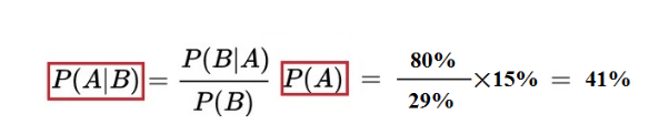
It can be calculated that the probability of the vehicle being involved in the accident is blue when there are witnesses = 41%. It can be seen from the results that the corrected conditional probability of “the vehicle causing the accident is blue” is 41%, which is much higher than the prior probability of 15%.
Example 3: In the formula (2), the definition of “prior” and “posterior” is a kind of “conventional”, which is relatively speaking. The posterior probability calculated in the previous time can be used as the prior probability of the subsequent time. Combined with the new observed data, a new posterior probability is obtained. Therefore, using the Bayesian formula, the probability model can be revised successively for some unknown uncertainty and the final objective result can be obtained.
Or to put it another way, sometimes it can be said that observers may revise their subjective “confidence” in an event based on the Bayesian formula and increasing data.
Take the example of a coin toss, which is generally considered to be “fair”. However, there are too many cases of fraud, and the results need to rely on data to speak.
For example, suppose the proposition A is: “This is a fair coin”, and the observer’s confidence in this proposition is represented by P(A). If P(A)=1, it means that the observer firmly believes that the coin is fair; the smaller the P(A), the lower the observer’s trust in the fairness of the coin; if P(A)=0, it means that the observer The person believes that the coin is unfair, for example, a counterfeit “right” coin with both sides marked “heads”. If B is used to represent the proposition “This is a straight coin”, then P(B) = 1- P(A).
Let’s see how to update the observer’s “trust” model P(A) according to the Bayesian formula.
First of all, he assumes a “prior trust degree”, such as P(A)=0.9, 0.9 is close to 1, which means that he is more inclined to believe that the coin is fair. Then, toss a coin once to get “Positive Head”, he updates P(A) to P(A|H) according to the Bayesian formula:
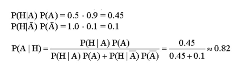
The updated posterior probability P(A|H) = 0.82, then throw it again and get a head (H), the new updated value after two heads is P(A|HH) = 0.69, after three heads The updated value is P(A|HHH) = 0.53. Throwing it down like this, if you get heads for 4 consecutive times, the new update value is P(A|HHHH) = 0.36. At this time, the observer’s confidence in the coin being a fair coin has decreased a lot. Since the trust level dropped to 0.5, he has already doubted the fairness of the coin. After 4 consecutive positives, he is more inclined to think that The coin is most likely a counterfeit with two heads!
From the above few examples, we have a preliminary understanding of Bayes’ theorem and its simple applications.
The significance of Bayes’ theorem
Bayesian theorem is Bayesian’s greatest contribution to probability theory and statistics, but at that time, Bayesian “reverse probability” research and derived Bayesian theorem seemed plain and unremarkable, Bayesian is also little-known. Now it seems that this should not be the case at all. The significance of the Bayesian formula is the method of detecting unknown probabilities as shown in Example 3. People first have a priori guess, and then combine the observed data to correct the priori and get a more reasonable posterior probability. That is to say, when you cannot accurately know the essence of a certain thing, you can rely on experience to approach the state of the unknown world step by step, so as to judge its essential attributes. In fact, its thought is far beyond the understanding of ordinary people, and perhaps Bayes himself did not know enough about it during his lifetime. Because of such an important result, he did not publish it during his lifetime. It was published by a friend in 1763 after his death. Later, Laplace proved a more general version of Bayes’ theorem and used it in celestial mechanics and medical statistics. Today, Bayes’ theorem is the basic framework of machine learning commonly used in today’s artificial intelligence [3] .
Bayes’ theorem was contrary to the classical statistics at that time, and even seemed a bit “unscientific”. Therefore, it has been hidden in the snow for many years and is not welcomed by scientists. As can be seen from Example 3 in the previous section, the application method of Bayesian theorem is based on subjective judgment. First, a value is guessed subjectively, and then it is continuously revised according to empirical facts, and finally the essence of the objective world is obtained. In fact, this is exactly the scientific method, and it is also the method for human beings to understand the world (learn) starting from children. Therefore, it can be said that one of the keys to the prosperity of artificial intelligence research in recent years comes from the “marriage” of classical computing technology and probability statistics. The Bayesian formula in it summarizes the principles of people’s learning process. If it is combined with big data training, it is possible to more accurately simulate the human brain, teach machines to “learn”, and accelerate the progress of AI. Judging from the current situation, it is also true.
How do machines learn?
Teach machine learning, what to learn? In fact, it is to learn how to process data, which is what adults teach children to learn: to dig out useful information from a large amount of sensory data. If it is described in the language of mathematics, it is to model from the data and abstract the parameters of the model [4] .
The task of machine learning includes the main functions such as “regression”, “classification”, and so on. Regression is a commonly used method in statistics. The purpose is to solve the parameters of the model in order to “return” the true colors of things. Classification is also an important part of machine learning. “Sorting things into categories” is also the first step in human beings’ cognition of the world since infants. Mothers teach their children: this is a dog, that is a cat. This learning method belongs to “classification” and is “supervised” learning under the guidance of mothers. Learning can also be “unsupervised”. For example, children see “birds and airplanes flying in the sky” and “fish and submarines swimming in the water”, etc., and they can naturally divide these things into There are two categories of “flying objects” and “swimming objects”.
Bayesian formula can also be used to classify data, an example is given below.
Suppose we tested the data of 1000 fruits, including the following three characteristics: shape (long?), taste (sweet?), color (yellow?), there are three types of these fruits: apples, bananas, or pears, as shown in Figure 2 Show. Now, using a Bayesian classifier, how would it classify a new given fruit? For example, this fruit has all three characteristics: long, sweet, and yellow. Then, the Bayesian classifier should be able to give the probability that this new data fruit is each fruit based on the known training data.
First of all, what can we get from the data of 1000 fruits?
- Of these fruits, 50% are bananas, 30% are apples, and 20% are pears. That is, P(banana) = 0.5, P(apple) = 0.3, P(pear) = 0.2.
- Of the 500 bananas, 400 (80%) are long, 350 (70%) are sweet, and 450 (90%) are yellow. That is, P(long|banana) = 0.8, P(sweet|banana) = 0.7, and P(yellow|banana) = 0.9.
- Of the 300 apples, 0 (0%) are long, 150 (50%) are sweet, and 300 (100%) are yellow. That is, P(long|apple) = 0, P(sweet|apple) = 0.5, and P(yellow|apple) = 1.
- Of the 200 pears, 100 (50%) are long, 150 (75%) are sweet, and 50 (25%) are yellow. That is, P(long|pear) = 0.5, P(sweet|pear) = 0.75, P(yellow|pear) = 0.25.
In the above description, P(A|B) means “the probability of occurrence of A when condition B is established”. probability of occurrence.
The so-called “naive Bayesian classifier”, the word “naive” means that the information expressed in the data is independent of each other, in the specific case of this example, that is to say, the fruit’s “long, sweet, yellow “These three characteristics are independent of each other because they describe the fruit’s shape, taste and color, respectively, and are not related to each other. The term “Bayesian” indicates that this type of classifier uses the Bayesian formula to calculate the posterior probability, namely: P(A|new data) = P(new data|A) P(A)/P(new data ).
The “new data” here = “long sweet yellow”. The following calculates the probability that the fruit is a banana, an apple, or a pear under the condition of “long sweet yellow”. For bananas:
P(banana|long sweet yellow) = P(long sweet yellow|banana) P(banana)/ P(long sweet yellow)
The first item on the right side of the equation: P(long sweet yellow|banana) = P(long|banana) * P(sweet|banana) * P(yellow|banana) = 0.80.70.9 = 0.504.
In the above calculation, P (long sweet yellow|banana) is written as the product of three probabilities because the features are independent of each other.
Finally, it is obtained: P (banana|long sweet yellow) = 0.504*0.5/ P (long sweet yellow) = 0.252/ P (long sweet yellow).
A similar method is used to calculate the probability of apples: P(long sweet yellow|apple) = P(long|apple)P(sweet|apple) * P(yellow|apple) = 00.5*1 = 0. P(apple|long sweet yellow) = 0.
For pears: P(long sweet yellow|pear) = P(long|pear)P(sweet|pear) * P(yellow|pear) = 0.50.75*0.25 = 0.09375. P(pear|long sweet yellow) = 0.01873/ P(long sweet yellow).
Denominator: P (long sweet yellow) = P (long sweet yellow | banana) P (banana) + P (long sweet yellow | apple) P (apple) + P (long sweet yellow | pear) P (pear) = 0.27073
Finally available: P (banana|long sweet yellow) = 93%
P(apple|long sweet yellow) = 0
P(pear|long sweet yellow) = 7%
So when you give me a long, sweet, yellow fruit, in this case a Bayesian classifier trained on 1000 fruits concludes that this new fruit cannot be an apple (probability 0 %), there is a small probability (7%) that it is a pear, and the greatest probability (93%) is a banana.
The mysteries of deep learning
Look again, how do children learn to recognize dogs and cats? It is because his mother took him to see all kinds of dogs and cats, and many times of experience made him know many characteristics of dogs and cats, so he formed his own judgment method and divided them into two categories: “cat” and “dog”. kind. Scientists use similar methods to teach machine learning. For example, it might be possible to tell cats and dogs apart by their ears: “dogs have long ears, cats have short ears,” and “cat ears point up, dog ears point down.” According to the characteristics of these two “cats and dogs”, the obtained data is drawn in a plane diagram, as shown in Figure 3b. At this time, it is possible to use a straight line AB in Figure 3b to easily separate cats and dogs by these two features. Of course, this is just an example of simply explaining “characteristics”, and it does not necessarily distinguish cats from dogs.
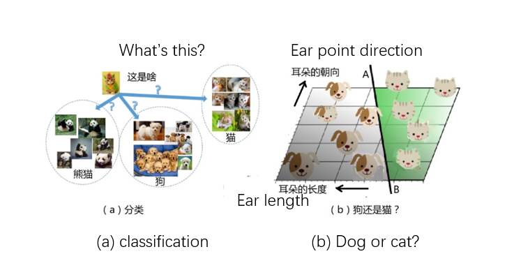
All in all, the machine can make a linear division of the area according to a certain “feature”. So, where should this line be drawn? This is what the “training” process needs to address. In the machine model, there are some parameters called “weights” w1, w2, w3, …, and the process of “training” is to adjust these parameters so that the straight line AB is drawn at the correct position and points in the correct direction. In the above “cat and dog” example, the output may be 0, or 1, representing a cat and a dog, respectively. In other words, the so-called “training” means that the mother is teaching the child to recognize cats and dogs. For the AI model, it means inputting a large number of photos of “cats and dogs”. Known answer.
The trained AI model can be used to identify photos of cats and dogs without marked answers. For example, for the above example: if the data falls on the left side of the line AB, output “dog”, and on the right side output “cat”.
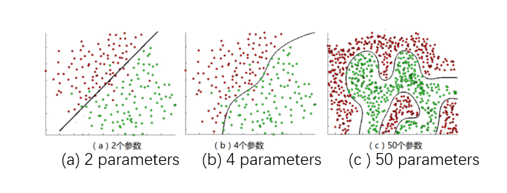
Figure 3b expresses a very simple situation. In most cases, the two types cannot be completely separated by a straight line. For example, the increasingly complex situations shown in Figure 4a, Figure 4b, and Figure 4c are not many. talked about.
discriminant and generative
Supervised learning models in machine learning can be divided into two types: discriminative models and generative models. From the previous description, we understand how machines “classify”. From the names of these two learning methods, it can be simply understood that: the discriminative model is more about the classification problem, while the generative model is to generate a sample that meets the requirements.
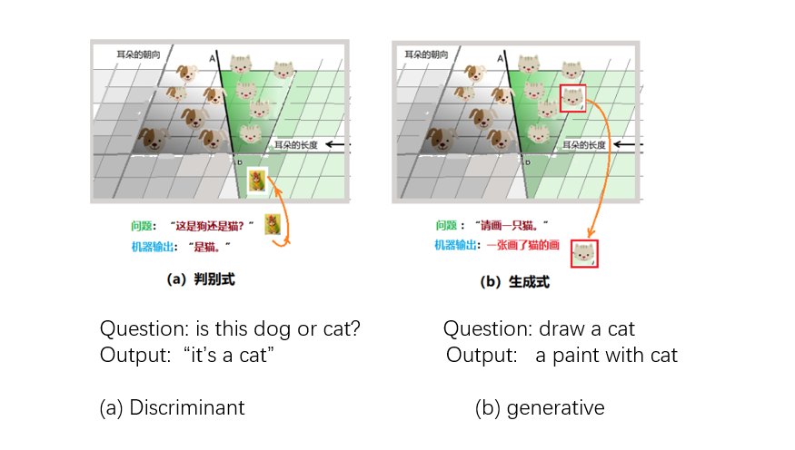
Also use the example of recognizing “cats and dogs” and use mothers to teach children to compare. After showing the child many samples of cats and dogs, the mother pointed to a cat and asked the child, what is this? The child makes a judgment “it’s a cat” after recalling, which is the discriminant formula. The child was very happy when he got the answer right. He picked up the pen and drew an image of a cat in his mind on the paper. This is the generative expression. The work of the machine is also similar, as shown in Figure 5. In the discriminant model, the machine looks for the boundary line needed for discrimination to distinguish different types of data instances; the generative model can distinguish between dogs and cats, and finally draws a “new “Animal photos: dog or cat.
In the language of probability: let the variable Y represent the category and X represent the observable feature. The discriminant model is to let the machine learn the conditional probability distribution P(Y|X), that is, the probability that the category is Y under a given feature X; in the generative model, the machine establishes a joint probability P(X,Y) for each “category” , thus generating “new” samples that look like a certain type.
For example, the category Y is “cat, dog” (0,1), and the feature X is the “up and down” (1,2) of the ear. Suppose we only have 4 photos as shown in the figure: (x,y)= { (1,1),(1,0),(2,0),(2,0)}
The discriminant is modeled by the conditional probability P(Y|X), and the dividing line is obtained (the red dotted line in the lower left figure); the generative formula is modeled by the joint probability P(X,Y) for each category, there is no dividing line, but the division The location interval of each type in the data space is shown (the red circle in the lower right figure). Both methods work according to the probabilities given by different models. The discriminant is simpler and only cares about the dividing line; while the generative model needs to model each category, and then calculate the posterior probability of the sample belonging to each category through the Bayesian formula. Generative information is rich and flexible, but the learning and calculation process is complex and the amount of calculation is large. If only classification is done, the amount of calculation will be wasted.
A few years ago, the discriminative model was more popular, because it used a more direct way to solve the problem, and it has already been used in many applications, such as the classification of spam and normal mail. AlphaGo in 2016 is also a typical example of discriminative application for decision-making.
Features of ChatGPT
If you have chatted with ChatGPT, you will be amazed at its wide range: creating poetry, generating code, drawing and drawing, writing papers, it seems to be good at everything, and it is omnipotent. What gave it such a powerful skill?
From the name of ChatGPT, we know that it is a “generative pre-training transformation model” (GPT). There are three meanings here: “generative”, “pre-training”, and “transformation model”. The first word indicates that it uses the generative modeling method described above. Pre-training means that it has been trained many times. The transformation model is translated from the English word for “transformer”. The transformer transformer was launched by a team at Google Brain in 2017 and can be applied to tasks such as translation and text summarization. It is now considered to be the model of choice for NLP dealing with sequential input data problems such as natural language.
If you ask ChatGPT yourself, “What is it?” Questions, generally speaking, it will tell you that it is a large AI language model, which refers to the transformer.
This type of language model, in layman’s terms, is a machine that can “text solitaire”: input a piece of text, the converter outputs a “word”, and performs a “reasonable continuation” of the input text. (Note: Here I said that the output is a “word”, which is actually a “token”, which may have different meanings for different languages. Chinese can be “character”, and English may be “root”.)
In fact, language is originally “Solitaire”. We might as well think about the process of children learning language and writing. They also learn how to say a sentence after listening to adults say various sentences many times. Learning to write is also similar. Some people say: “If you are familiar with three hundred Tang poems, you can chant poems even if you don’t know how to write them.” After reading a lot of other people’s articles, when students start learning to write, they will always imitate. Learned “Word Solitaire”.
So in fact, what the language model does sounds extremely simple, basically just repeatedly asking “what should the next word of the input text be?”, as shown in Figure 7, after the model chooses to output a word, Add this word to the original text, enter the language model as input, and ask the same question “what is the next word?”. Then, output, add text, input, select… repeat the cycle until a “reasonable” text is generated.
Whether the text generated by the machine model is “reasonable” or unreasonable, the most important factor is of course the quality of the “generative model” used, and then the “pre-training” effort. Inside a language model, given an input text, it produces a sorted list of words that might appear next, along with the probabilities associated with each word. For example, if the input is “Spring Breeze”, there are many, many possible next “words”. Let’s just list 5 for now, which can be “blowing 0.11, warming 0.13, re-0.05, reaching 0.1, dancing 0.08” and so on, after each word The numbers in represent the probability of its occurrence. In other words, the model is given a (very long) list of words with probabilities. So, which one should you choose?
If you choose the one with the highest probability every time, it should not be “reasonable”. Let’s think about the process of students learning to write. Although they are also “solitaire”, different people and different times have different ways of connecting. Only in this way can we write a variety of different styles and creative articles. Therefore, the machine should also be given the opportunity to randomly select different probabilities in order to avoid monotony and produce colorful and interesting works. Although it is not recommended to choose the one with the highest probability every time, it is better to choose the one with high probability and make a “reasonable model”.
ChatGPT is a large-scale language model. This “big” is firstly reflected in the number of weight parameters of the model neural network. Its number of parameters is a key factor in determining its performance. These parameters need to be preset before training, and they can control the syntax, semantics and style of the generated language, as well as the behavior of language understanding. It also controls the behavior of the training process, and the quality of the generated language.
OpenAI’s GPT-3 model has 175 billion parameters, ChatGPT is GPT-3.5, and the number of parameters should be more than 175 billion. These parameters refer to the parameters that need to be preset before training the model. In practical applications, it is usually necessary to determine the appropriate number of parameters through experiments to obtain optimal performance.
These parameters are modified over thousands of training sessions to produce a good neural network model. It is said that the cost of GPT-3 training is 4.6 million US dollars, and the total training cost is 12 million US dollars.
As mentioned above, ChatGPT’s specialty is generating text “similar to human writing”. But a thing that can generate a grammatical language may not be able to perform other types of work such as mathematical calculations, logical reasoning, etc., because the expressions in these fields are completely different from natural language texts, which is why it is tested in mathematics. The reason for repeated failures.
Also, one often finds ChatGPT “seriously talking nonsense” jokes. The reason is not difficult to understand, the main problem is the bias of training. Something it hadn’t heard at all, of course it couldn’t give a correct answer. There are also problems caused by polysemous words, which also confuse the machine model. For example, it is said that when someone asked ChatGPT “What is the hook three strands four strings five”, it replied solemnly: “This is the tuning method of a musical instrument called ‘qin’ in ancient China, and then made up a lot of words , It’s hilarious.
In short, ChatGPT basically succeeded as soon as it came on the field, and it was a victory. This is also a victory of probability theory and Bayesian victory.